基于夏普比率的交易策略
本文探讨了一种使用夏普比率生成多头和空头信号的特定量化策略,旨在利用风险调整后表现强劲的时期。
一键发币: x402兼容 | Aptos | X Layer | SUI | SOL | BNB | ETH | BASE | ARB | OP | Polygon | Avalanche
以太坊和比特币等加密货币以其高波动性而闻名,这为交易者带来了机遇和巨大的风险。驾驭这些动荡的市场通常需要严谨的方法。量化交易策略依靠数学模型和历史数据来做出交易决策,它提供了一个这样的框架。
本文探讨了一种使用夏普比率生成多头和空头信号的特定量化策略,旨在利用风险调整后表现强劲的时期。我们将分解其逻辑,逐步分析其在 Python 中的实现,并讨论评估此类策略的关键考虑因素。
1、设置:导入库
首先,我们导入必要的 Python 库:
import yfinance as yf       # To download historical market data from Yahoo Finance
import pandas as pd         # For data manipulation and analysis (DataFrames)
import numpy as np          # For numerical operations (like square root)
import matplotlib.pyplot as plt # For plotting the results
说明:我们需要 yfinance 获取价格数据,使用 pandas 在类似表格的结构(DataFrame)中高效地处理数据,使用 numpy 进行数学计算,并使用 matplotlib 可视化策略的效果。
2、策略参数
我们定义控制策略行为的核心参数:
# Parameters
symbol = "ETH-USD"          # The asset we want to trade
start_date = "2018-01-01"   # Start date for historical data
end_date = "2025-04-17"     # End date for historical data (use current date for latest)
window = 30                 # Rolling window (in days) for Sharpe Ratio calculation
upper_threshold = 2.0       # Sharpe Ratio threshold to trigger a long signal
lower_threshold = -2.0      # Sharpe Ratio threshold to trigger a short signal
hold_days = 7               # Maximum number of days to hold a position
stop_loss_pct = 0.20        # Stop-loss percentage (e.g., 0.20 = 20%)
说明:这些变量可以轻松调整策略。我们指定加密货币对(ETH-USD)、回测的日期范围、夏普计算的回溯期(窗口)、触发交易的阈值、任何交易的最大持有天数以及用于风险管理的止损百分比。
3、数据采集与准备
我们下载历史价格数据并计算基本收益:
# 1) Download data
df = yf.download(symbol, start=start_date, end=end_date, progress=False)
# Clean column names (sometimes yfinance returns multi-level columns)
df.columns = [col.lower() for col in df.columns] # Make column names lowercase
# 2) Calculate daily returns
df["return"] = df["close"].pct_change() # Calculate daily percentage change in closing price
说明:我们使用 yf.download 获取以太坊的开盘价、最高价、最低价、收盘价、调整收盘价和成交量数据。我们简化列名,然后根据收盘价从一天到下一天的百分比变化计算每日收益。此收益序列是我们夏普系数计算的基础。
4、计算滚动夏普比率
这是核心信号生成步骤。我们计算滚动窗口内的夏普比率:
# 3) Compute rolling Sharpe (annualized)
# Calculate rolling mean return and rolling standard deviation
rolling_mean = df["return"].rolling(window).mean()
rolling_std = df["return"].rolling(window).std()
# Calculate annualized Sharpe Ratio
# Note: np.sqrt(365) is arguably more appropriate for crypto (24/7 market)
df["rolling_sharpe"] = (rolling_mean / rolling_std) * np.sqrt(252)
说明:对于每一天,我们回顾指定的窗口(30 天)。我们计算该期间的平均日收益 (rolling_mean) 和日收益的标准差 (rolling_std)。夏普比率等于 rolling_mean / rolling_std。我们将其乘以每年交易日的平方根,进行年化(此处使用 np.sqrt(252);对于加密货币,np.sqrt(365) 通常更合适)。数值越高,表明近期风险调整后的收益越好。
5、生成交易信号
根据计算出的夏普比率,我们生成原始入场信号:
# 4) Generate entry signals based on thresholds
df["signal"] = 0 # Default signal is neutral (0)
df.loc[df["rolling_sharpe"] > upper_threshold, "signal"] = 1  # Go Long if Sharpe > upper
df.loc[df["rolling_sharpe"] < lower_threshold, "signal"] = -1 # Go Short if Sharpe < lower
说明:我们创建一个新的信号列,初始值为全零。如果某天的 rolling_sharpe 高于 upper_threshold (2.0),我们将 t 设置为将信号设置为 1(买入)。如果低于 lower_threshold (-2.0),我们将信号设置为 -1(做空)。否则,信号保持为 0(不执行任何操作)。
6、准备回测
在运行模拟之前,我们调整信号时序并初始化变量:
# 5) Prepare for Backtest: Shift signals to avoid lookahead bias
# We use yesterday's signal to trade on today's price
df['signal_shifted'] = df['signal'].shift(1).fillna(0)
# Initialize backtest variables
position = 0                # Current position: 1=long, -1=short, 0=flat
entry_price = 0.0           # Price at which the current position was entered
days_in_trade = 0           # Counter for days held in the current trade
equity = 1.0                # Starting equity (normalized to 1)
equity_curve = [equity]     # List to store equity values over time
说明:
- df['signal'].shift(1):这一项至关重要。它将信号向前移动一天。这意味着,使用截至 T 日结束的数据生成的信号将用于在 T+1 日做出交易决策。这可以避免前瞻偏差。.fillna(0) 处理没有先前信号的第一天。
- 我们将持仓初始化为 0(持平),跟踪当前持仓的 entry_price 和 days_in_trade,假设权益为 1,并创建一个列表 equity_curve 来记录该权益随时间的变化。
7、回测引擎循环
此循环逐日模拟策略:
# 6) Backtest Engine Loop
# Start loop from 'window' index to ensure enough data for rolling calculation and shift
for i in range(window, len(df)):
    idx = df.index[i]           # Current date
    row = df.iloc[i]            # Current day's data row
    price = row["close"]        # Use today's close price for trading action (simplification)
    sig = row["signal_shifted"] # Use *yesterday's* calculated signal
    # --- Check Exits First ---
    if position != 0: # Are we currently in a trade?
        days_in_trade += 1
        # Calculate potential return if we closed the trade *right now*
        current_return_pct = (price / entry_price - 1) * position
        # Check Stop Loss: Did the trade lose more than stop_loss_pct?
        if current_return_pct <= -stop_loss_pct:
            equity *= (1 - stop_loss_pct) # Apply the max loss percentage
            position = 0 # Exit position
        # Check Holding Period: Have we held for the max number of days?
        elif days_in_trade >= hold_days:
            equity *= (1 + current_return_pct) # Realize the profit/loss
            position = 0 # Exit position
    # --- Check Entries Second ---
    # Can only enter if currently flat (position == 0) and there's a non-zero signal
    if position == 0 and sig != 0:
        position = sig            # Enter long (1) or short (-1)
        entry_price = price       # Record entry price (using today's close)
        days_in_trade = 0         # Reset trade duration counter
    # Append the *current* equity value to the curve after all checks/trades
    equity_curve.append(equity)
说明:
循环在计算所需的初始窗口期后开始逐日迭代。
在循环内部,它首先检查我们是否已在交易中(position != 0)。
如果是,它会递增 days_in_trade 的值,并根据 entry_price 和当日价格计算 current_return_pct。
然后,它会检查退出条件:止损 — 如果 current_return_pct 的亏损大于或等于 stop_loss_pct,则平仓,净值减少 stop_loss_pct。
持有期:如果 days_in_trade 达到 hold_days,则平仓,并将已实现的盈亏 (current_return_pct) 计入净值。
如果我们没有交易 (position == 0),它会检查是否有新的入场信号 (sig != 0)。如果是,它会设置仓位,记录 entry_price,并重置 days_in_trade。
最后,它会将可能更新的净值添加到当天的 equity_curve 列表中。
8、后处理和对齐
我们将计算出的权益曲线与 DataFrame 中的相应日期对齐:
# 7) Align Equity Curve with DataFrame
# Remove the initial equity point (1.0) as it corresponds to the day *before* the loop starts
equity_curve_series = pd.Series(equity_curve[1:], index=df.index[window:])
# Add the equity curve to the DataFrame
df["equity"] = equity_curve_series
说明:equity_curve 列表开头包含一个额外的点(初始 1.0)。我们删除它,并使用 DataFrame 中与回测周期(从 window 索引开始)对应的日期创建一个 Pandas Series。然后,该权益序列将作为新列添加到 DataFrame df 中。
9、绘制结果
最后,我们将业绩可视化:
# 8) Plot Equity Curve vs. Buy-and-Hold
plt.figure(figsize=(12, 7)) # Create a figure for the plot
# Plot the strategy's equity curve
plt.plot(df.index, df["equity"], label="Sharpe Strategy Equity")
# Plot the normalized price of the asset (Buy and Hold)
# Normalize by dividing by the first closing price in the backtest period
buy_hold = df['close'] / df['close'].iloc[window] # Adjust starting point
plt.plot(buy_hold.index, buy_hold, label=f"Buy & Hold {symbol}", alpha=0.7)
# Add plot titles and labels
plt.title(f"Equity Curve: {symbol} {window}-day Sharpe Strategy")
plt.ylabel("Equity (Normalized)")
plt.xlabel("Date")
plt.legend() # Show the legend
plt.grid(True) # Add a grid for readability
plt.show() # Display the plot
说明:此代码使用 matplotlib 生成图表,显示该策略随时间变化的权益曲线。为了进行比较,它还绘制了在同一时期内简单买入并持有 ETH-USD 的表现(标准化,起始值为 1)。这种直观的比较有助于评估该策略的相对表现和风险状况。
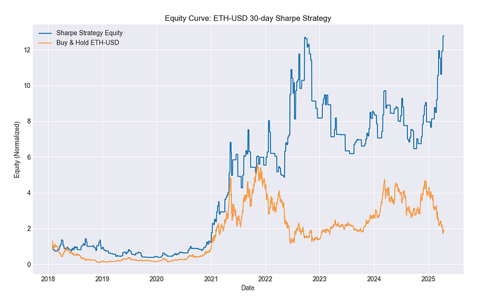
结果解读及重要注意事项
输出图可视化了假设的资本增长情况。将该策略的权益曲线与标准化的以太坊价格进行比较,有助于评估该策略在测试期间是否实现了增值(优于买入并持有策略),并且可能具有不同的风险特征(例如,更低的回撤)。
然而,了解其局限性至关重要:
- 交易成本和滑点:代码忽略了交易费用和滑点,这会降低实际利润。
- 参数优化(过度拟合):参数可能根据历史数据进行调整,未来可能无法正常工作。
- 数据频率:每日数据掩盖了日内风险;止损可能在比收盘价更差的价格触发。
- 年化因子:对于加密货币,使用 np.sqrt(365) 可能更准确。
- 市场机制:过往表现并不能保证未来结果;该策略在不同的市场条件下可能会失效。
- 简化:使用收盘价执行是一种近似值。
10、结束语
这种基于夏普比率的策略提供了一种结构化的、量化的加密货币交易方法。虽然回测(采用修正后的逻辑,避免了前瞻偏差)提供了一些见解,但本代码和文章仅供参考,不构成财务建议。在实际交易中,需要在投入资金之前考虑成本、进行严格的过拟合测试以及稳健的风险管理。
原文链接:Crypto Trading Strategy using the Sharpe Ratio with Python Code
DefiPlot翻译整理,转载请标明出处
免责声明:本站资源仅用于学习目的,也不应被视为投资建议,读者在采取任何行动之前应自行研究并对自己的决定承担全部责任。