基于机器学习的Crypto交易算法

一键发币： SOL | BNB | ETH | BASE | Blast | ARB | OP | POLYGON | AVAX | FTM | OK

机器学习已成为算法交易策略领域的工具，利用数值、分类和序数数据来构建现实世界的简化模型。本文将利用 pycgapi（一种用于访问 CoinGecko API 的非官方 Python 包装器）来获取关键市场数据并构建算法交易策略。

通过将 Python 的计算能力与 CoinGecko 提供的丰富数据集相结合，我们将应用机器学习技术来开发、测试和实施加密货币领域的算法交易策略。更具体地说，我们将专注于利用称为分层风险平价 (HRP) 投资组合策略的无监督机器学习算法。

1、开发环境准备

在本节中，我们概述了学习本教程所需的必要背景知识、软件和库，以及设置环境的步骤。

1.1 背景知识

• Python 熟练程度：你应该熟悉变量、循环和函数等基本编程概念，以及使用库和处理数据等更高级的主题。
• 了解金融市场：对金融市场和工具（尤其是加密货币）有基本的了解将大有裨益。
• 数学和统计学：建议了解基本的数学和统计学知识，以便学习本教程的财务分析部分。

1.2 Google Colab

本教程使用 Google Colab，这是一项免费的云服务，允许你在浏览器中编写和执行 Python，无需任何配置，可以访问免费的 GPU，并且易于共享。使用 Google Colab 无需本地设置，并确保每个人都可以访问相同的计算环境，从而更轻松地学习和排除故障。

确保将 Google Colaboratory 添加到你的 Google Drive 帐户的关联应用中，如下所示。在你的 Google Drive 帐户中，点击“+新建”>“更多”。如果在菜单中没有看到 Google Colaboratory，请点击“+连接更多应用”。通过 Google Drive 访问 Google Colab

搜索“Google Colaboratory”，然后安装。 Google Colaboratory

💡专业提示：在此处关注本文的 Google Colab 版本。我还建议你通过查看他们的精选笔记本来熟悉 Colab 界面和功能。

1.3 配置 API 密钥

为了访问加密数据和自动化交易，我们将使用 CoinGecko 和 Alpaca API。

• CoinGecko API：用于获取加密货币市场数据。
• Alpaca API：在 Alpaca 平台上启用自动交易。

为这些服务设置 API 密钥使我们能够以编程方式检索实时加密数据并执行交易，这是算法交易的重要组成部分。

要获取你的 API 密钥：

• 登录你的 CoinGecko 帐户并转到开发者仪表板。单击“添加新密钥”。存储在安全的位置。
• 登录你的 Alpaca 帐户并导航到 Paper Trading Dashboard。单击 API 密钥框中的“生成”。创建后，将显示你的 API 密钥和密钥。此时安全地保存这些密钥至关重要，因为密钥不会再次显示。如果丢失了密钥，则需要生成一对新密钥。

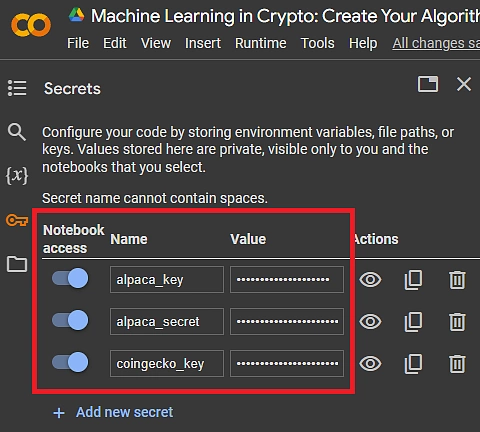
1.4 将 API 密钥存储在 Google Colab Secrets 中

在 Google Colab 中，单击左侧菜单中的密钥图标。

输入每个密钥的名称，将密钥粘贴为值，并授予笔记本对每个密钥的访问权限。

要访问财务数据，请按如下方式配置你的 API 密钥：

from google.colab import userdata
coingecko_key = userdata.get('coingecko_key')
alpaca_key = userdata.get('alpaca_key')
alpaca_secret = userdata.get('alpaca_secret')

1.5 安装所需的库

本教程使用几个自定义 Python 库：

• pycgapi：用于访问 CoinGecko API 获取加密货币数据的客户端。
• alpaca-py：Alpaca 交易 API 的官方 Python 库，支持自动交易策略。
• PyPortfolioOpt：提供投资组合优化技术，例如均值方差优化。
• bt：用于测试和开发量化交易策略的灵活 Python 回测框架。

在 Google Colab 单元中运行以下命令来安装它们：

%%capture
!pip install alpaca-py
!pip install PyPortfolioOpt
!pip install git+https://github.com/nathanramoscfa/bt.git
!pip install git+https://github.com/nathanramoscfa/pycgapi.git@legacy-0.1.5

1.6 导入库

安装完成后，使用以下代码导入必要的库。这些库将帮助我们处理数据、执行财务分析、构建投资组合并运行机器学习算法。

import warnings
warnings.simplefilter(action='ignore', category=FutureWarning)

import math
import time
import pandas as pd
import numpy as np
import matplotlib.pyplot as plt
import matplotlib.dates as mdates
from tqdm import tqdm
from datetime import datetime
from typing import Any, Tuple

from sklearn.preprocessing import StandardScaler
from scipy.cluster.hierarchy import dendrogram, linkage
from scipy.stats import norm, t, ttest_1samp

from pycgapi import CoinGeckoAPI
from alpaca.trading.client import TradingClient
from alpaca.trading.requests import GetAssetsRequest, MarketOrderRequest
from alpaca.trading.enums import AssetClass, OrderSide, TimeInForce

from pypfopt.risk_models import CovarianceShrinkage
from pypfopt.hierarchical_portfolio import HRPOpt
from pypfopt.expected_returns import returns_from_prices

import bt
import ffn

2、初始化 API 客户端

现在，让我们设置与 CoinGecko 和 Alpaca API 交互所需的客户端。这些客户端充当我们的 Python 代码和外部服务之间的桥梁，使我们能够获取实时加密货币数据并以编程方式执行交易。

对于 CoinGecko，我们将使用专业 API 密钥，因为所需的数据量较大，并且要以更高的速率限制运行。

对于 Alpaca，你将需要纸质（模拟交易）或实时交易 API 密钥，具体取决于你的交易模式偏好。

# Configuration Variables
pro_api = True  # Set to True if using a paid CoinGecko API key
paper = True  # Set to False for live trading on Alpaca

2.1 初始化 CoinGecko API 客户端

为了与 CoinGecko API 交互，我们初始化一个客户端，该客户端将请求加密货币数据。这些数据对于在我们的算法中做出明智的交易决策至关重要。

# Initialize the CoinGecko API client
cg = CoinGeckoAPI(coingecko_key, pro_api=pro_api)

# Check API server status
try:
    status = cg.status_check()
    print("CoinGecko API Server Status:", status)
except Exception as e:
    print("Error checking CoinGecko API status:", e)

运行结果输出如下：

CoinGecko API Server Status: {'gecko_says': '(V3) To the Moon!'}

2.2 初始化 Alpaca API 客户端

为了执行交易，我们使用 Alpaca API 客户端。根据我们之前的纸质设置，此客户端将配置为纸质交易（模拟）或实时交易

# Initialize the Alpaca trading client
trading_client = TradingClient(alpaca_key, alpaca_secret, paper=paper)

# Output initialization status
trading_mode = "Paper Trading" if paper else "Live Trading"
print(f"Alpaca Trading Client Initialized: {trading_mode}")

运行结果输出如下：

Alpaca Trading Client Initialized: Paper Trading 

3、投资领域

在本节中，我们将 Alpaca 中可交易的加密货币代码与 CoinGecko 中相应的代币 ID 对齐。

这种对齐至关重要，因为 Alpaca 和 CoinGecko 对加密货币代码使用不同的格式。例如，Alpaca 使用“BTC/USD”等货币对，而 CoinGecko 通过代币 ID（例如“比特币”）识别加密货币。

通过协调这些格式，我们确保我们的策略仅考虑在 Alpaca 上可交易且在 CoinGecko 上有可用数据的加密货币。

3.1 Alpaca 上可交易的加密货币代码

首先，我们从 Alpaca 中检索所有可交易的加密货币代码，重点关注那些我们可以交易且在 CoinGecko 上有数据的加密货币。

# Get tradable crypto assets on Alpaca
search_params = GetAssetsRequest(asset_class=AssetClass.CRYPTO)
assets = trading_client.get_all_assets(search_params)
tradable_assets = pd.DataFrame([
    {'symbol': asset.symbol, 'tradable': asset.tradable}
    for asset in assets
]).set_index('symbol').sort_index()
print('Tradable Currency Pairs on Alpaca:\n')
print(tradable_assets.head())

运行上述代码的输出结果如下：

Tradable Currency Pairs on Alpaca:

           tradable
symbol             
AAVE/USD       True
AAVE/USDC      True
AAVE/USDT      True
AVAX/USD       True
AVAX/USDC      True

3.2 CoinGecko 的加密货币代码

接下来，我们将 Alpaca 的可交易代码与 CoinGecko 货币 ID 进行匹配，排除以“BTC”为基础货币的代码，重点关注以美元为基础的货币对。

# Store CoinGecko search results for tickers
search_results_dict = {}
for symbol in tqdm(tradable_assets.index):
    quote_currency, base_currency = symbol.split('/')
    if base_currency == 'USD' and tradable_assets.loc[symbol, 'tradable']:
        search_results = cg.search_coingecko(query=quote_currency)['coins']
        search_results_dict[symbol] = search_results

# Display search results
print(f"\n\nFound CoinGecko IDs for {len(search_results_dict)} assets.")

输出结果如下：

100%|██████████| 56/56 [00:09<00:00,  5.98it/s]
Found CoinGecko IDs for 20 assets.

3.3 收集 CoinGecko 代币 ID

我们从搜索结果中收集 CoinGecko 代币 ID，不包括稳定币，以专注于风险资产。

# Dictionary for storing found CoinGecko coin IDs
found_coin_ids = {
    key: value['id'].iloc[0] for key, value in search_results_dict.items()
}

# Sorting coin IDs
coin_ids = sorted(found_coin_ids.values())

# Define a list of stablecoins to exclude
stablecoins = ['tether', 'usd-coin']

# Filtering out stablecoins to focus on risky assets
risky_assets = [
    coin_id for coin_id in coin_ids if coin_id not in stablecoins
]

# Displaying CoinGecko Coin IDs
print('CoinGecko Coin IDs: \n')
for coin_id in risky_assets:  # Changed to risky_assets for relevant output
    print(coin_id)

输出结果如下：

CoinGecko Coin IDs: 

aave
avalanche-2
basic-attention-token
bitcoin
bitcoin-cash
chainlink
curve-dao-token
dogecoin
ethereum
litecoin
maker
polkadot
shiba-inu
sushi
tezos
the-graph
uniswap
yearn-finance

3.4 将 CoinGecko 代币 ID 映射到 Alpaca 交易符号

最后，我们在 CoinGecko 代币 ID 和 Alpaca 交易符号之间创建映射，以供后续交易逻辑使用。

# Create a dictionary mapping CoinGecko coin IDs to Alpaca trading symbols
ticker_mapping = {value: key.upper() for key, value in found_coin_ids.items()}

# Display ticker mapping
print("Ticker Mapping:\n")
for key, value in ticker_mapping.items():
    print(f"{key}: {value}")

输出结果如下：

Ticker Mapping:

aave: AAVE/USD
avalanche-2: AVAX/USD
basic-attention-token: BAT/USD
bitcoin-cash: BCH/USD
bitcoin: BTC/USD
curve-dao-token: CRV/USD
dogecoin: DOGE/USD
polkadot: DOT/USD
ethereum: ETH/USD
the-graph: GRT/USD
chainlink: LINK/USD
litecoin: LTC/USD
maker: MKR/USD
shiba-inu: SHIB/USD
sushi: SUSHI/USD
uniswap: UNI/USD
usd-coin: USDC/USD
tether: USDT/USD
tezos: XTZ/USD
yearn-finance: YFI/USD

4、获取实时和历史加密货币价格数据

使用 CoinGecko API 获取实时和历史加密货币价格数据。这对于我们交易策略的基础分析至关重要。

4.1 最早开始日期

评估历史数据的可用性，以确保我们选择的每种加密货币都有足够的历史数据供分析。使用此信息来评估您是否应该忽略最早开始日期太近的任何资产。

# Store each coin's earliest start date available
dfs = {}
for coin_id in tqdm(risky_assets):
    historical_data = cg.coin_historical_market_data(coin_id)
    first_date = historical_data.index[0].strftime('%Y-%m-%d')
    dfs[coin_id] = first_date

# Create dataframe of earliest start dates
start_dates = pd.DataFrame.from_dict(
    dfs, orient='index', columns=['Start Dates']
)

# Display earliest start dates
print(
    "\n\nEarliest Data Start Dates:\n\n",
    start_dates.squeeze().sort_values(ascending=False)
)

运行结果如下：

100%|██████████| 18/18 [00:13<00:00,  1.37it/s]

Earliest Data Start Dates:

 the-graph                2020-12-17
aave                     2020-10-03
avalanche-2              2020-09-22
uniswap                  2020-09-17
sushi                    2020-08-28
polkadot                 2020-08-19
curve-dao-token          2020-08-14
shiba-inu                2020-08-01
yearn-finance            2020-07-18
tezos                    2018-07-03
maker                    2017-12-20
chainlink                2017-11-09
bitcoin-cash             2017-08-02
basic-attention-token    2017-06-08
ethereum                 2015-08-07
dogecoin                 2013-12-15
bitcoin                  2013-04-28
litecoin                 2013-04-28
Name: Start Dates, dtype: object

4.2 当前价格

我们下载每种选定加密货币的当前市场价格，提供当前市场状况的视图。

# Get current prices for each coin
current_prices = cg.simple_prices(coin_ids)

# Mapping CoinGecko IDs to their corresponding Alpaca symbols
current_prices.index = current_prices.index.map(ticker_mapping)

# Display current prices
print("Current Prices:\n\n", current_prices)

输出结果如下：

Current Prices:

                     usd
AAVE/USD     102.730000
AVAX/USD      38.930000
BAT/USD        0.270338
BTC/USD    53392.000000
BCH/USD      270.950000
LINK/USD      18.960000
CRV/USD        0.599837
DOGE/USD       0.086983
ETH/USD     3152.620000
LTC/USD       71.140000
MKR/USD     2092.800000
DOT/USD        7.990000
SHIB/USD       0.000010
SUSHI/USD      1.570000
USDT/USD       1.000000
XTZ/USD        1.130000
GRT/USD        0.293909
UNI/USD       10.690000
USDC/USD       1.000000
YFI/USD     8325.900000

4.3 历史数据

我们下载每种选定加密货币的历史价格、市值和交易量数据。此数据集对于分析特定时期的市场行为至关重要。

# Get historical price, market cap, and volume for each coin
historical_data = cg.multiple_coins_historical_data(
    coin_ids, from_date='11-21-2022', to_date='02-21-2024'
)

# Create a copy of the historical data
historical_prices = historical_data['price'].copy()
historical_market_cap = historical_data['market_cap'].copy()
historical_volume = historical_data['total_volume'].copy()

# Display historical prices for selected columns
print('\n\nHistorical Prices:\n')
print(historical_prices.head().iloc[:, 3:8])

输出结果如下：

100%|██████████| 20/20 [00:12<00:00,  1.63it/s]

Historical Prices:

                                bitcoin  bitcoin-cash  chainlink  \
timestamp                                                          
2022-11-21 00:00:00+00:00  16304.076856    104.914267   5.780015   
2022-11-22 00:00:00+00:00  15814.335281    103.401328   5.878893   
2022-11-23 00:00:00+00:00  16171.628978    108.902578   6.386520   
2022-11-24 00:00:00+00:00  16608.009985    114.523828   6.721798   
2022-11-25 00:00:00+00:00  16596.035758    116.688272   6.833340   

                           curve-dao-token  dogecoin  
timestamp                                             
2022-11-21 00:00:00+00:00         0.512044  0.077732  
2022-11-22 00:00:00+00:00         0.501516  0.075124  
2022-11-23 00:00:00+00:00         0.633928  0.078690  
2022-11-24 00:00:00+00:00         0.688066  0.082338  
2022-11-25 00:00:00+00:00         0.689696  0.081835  

4.4 分类数据

最后，收集每种加密货币的分类信息。这些数据有助于了解不同加密货币类别的投资组合的多样化和风险敞口。

# Download and store categorical data for each coin
categories_dict = {}
for coin_id in tqdm(coin_ids):
    categories_dict[coin_id] = cg.coin_info(coin_id)['categories']

输出结果如下：

100%|██████████| 20/20 [00:09<00:00,  2.08it/s]

5、数据处理

本节概述了规范化、分析和可视化历史加密货币数据的步骤，为机器学习分析奠定了基础。

5.1 规范价格以进行比较分析

鉴于加密货币之间的价格差异很大，我们将所有价格标准化为 1 美元。这种方法通过平衡所有资产的初始投资来实现直接比较。

# Normalize prices to start at $1 for comparative analysis
historical_prices = historical_prices.rebase(1)

5.2 计算历史收益

我们根据标准化价格计算每日和累计收益，这是评估资产表现的关键指标。

# Calculate daily returns
historical_returns = historical_prices.pct_change().dropna()
historical_returns.index = historical_returns.index

# Calculate cumulative returns from daily returns
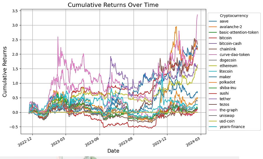
cumulative_returns = (1 + historical_returns).cumprod() - 1

5.3 可视化累计回报

可视化选定加密货币的累计回报不仅可以使数据变得生动，而且还有助于识别我们投资领域中表现突出和表现不佳的货币。

plt.figure(figsize=(10, 6))

# Plot cumulative returns for each cryptocurrency
for column in cumulative_returns.columns:
    plt.plot(cumulative_returns.index, cumulative_returns[column], label=column)

# Configure the x-axis to show dates correctly
plt.gca().xaxis.set_major_locator(mdates.MonthLocator(interval=3))
plt.gca().xaxis.set_major_formatter(mdates.DateFormatter('%Y-%m'))
plt.gcf().autofmt_xdate()  # Auto-format date labels
plt.title('Cumulative Returns Over Time', fontsize=16)
plt.xlabel('Date', fontsize=14)
plt.ylabel('Cumulative Returns', fontsize=14)
plt.legend(title='Cryptocurrency', loc='center left', bbox_to_anchor=(1, 0.5))
plt.grid(True, which='major', axis='both')  # Show major grid lines only
plt.tight_layout()
plt.show()

输出结果如下：

5.4 为机器学习准备数据

在进行机器学习分析之前，我们会对历史收益进行标准化。这种标准化可确保所有数据特征对分析的贡献均等，从而提高算法性能。

# Standardize historical returns
scale = StandardScaler()
historical_returns_scaled = pd.DataFrame(
    scale.fit_transform(historical_returns),
    columns=historical_returns.columns,
    index=historical_returns.index
).clip(lower=-3, upper=3)
print('Standardized Historical Returns:\n')
print(historical_returns_scaled.iloc[:, 3:8].head())

输出结果如下：

Standardized Historical Returns:

                            bitcoin  bitcoin-cash  chainlink  curve-dao-token  \
timestamp                                                                       
2022-11-22 00:00:00+00:00 -1.451238     -0.430926   0.357041        -0.492130   
2022-11-23 00:00:00+00:00  0.874272      1.263095   2.156707         3.000000   
2022-11-24 00:00:00+00:00  1.068304      1.223372   1.276908         1.909221   
2022-11-25 00:00:00+00:00 -0.155862      0.403770   0.343712         0.027544   
2022-11-26 00:00:00+00:00 -0.314597     -0.667662   0.001589        -0.341132   

                           dogecoin  
timestamp                            
2022-11-22 00:00:00+00:00 -1.023868  
2022-11-23 00:00:00+00:00  1.392055  
2022-11-24 00:00:00+00:00  1.359091  
2022-11-25 00:00:00+00:00 -0.205570  
2022-11-26 00:00:00+00:00  2.897963  

6、算法交易策略：分层风险平价

什么是分层风险平价 (HRP：Hierarchical Risk Parity)？

分层风险平价 (HRP) 方法由 López de Prado (2016) 提出，它使用分层聚类对资产进行分组，不是根据过去的回报，而是根据其价格序列的相似性。 HRP 旨在通过构建考虑资产之间层次关系的多元化投资组合，最大限度地减少传统投资组合优化方法中发现的估计误差。 HRP 的有效性在于它对市场变化的稳健性，通常优于传统的多元化技术。

6.1 分层风险平价

我们首先使用分层聚类来构建我们的资产。此方法从将每项资产作为单独的集群开始，并根据它们的相关性迭代合并它们。结果揭示了数据中的自然分组，有助于构建多元化投资组合。

# Prepare data for clustering
scaled_data = historical_returns_scaled.loc[:, risky_assets]

# Hierarchical clustering
linkage_matrix = linkage(scaled_data.T, method='ward')

# Dendrogram plot
plt.figure(figsize=(10, 6))
dendrogram(linkage_matrix, labels=scaled_data.columns, leaf_rotation=90)
plt.title('Asset Clusters by Hierarchical Clustering')
plt.xlabel('Cryptocurrency')
plt.ylabel('Distance')
plt.show()

输出结果如下：

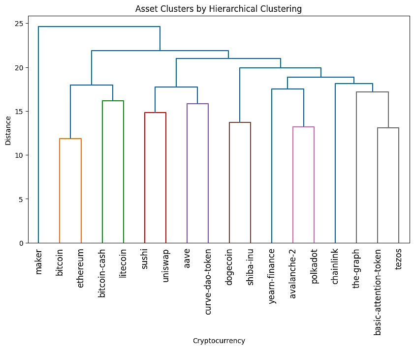
树状图显示了资产如何相互关联，分支越近，表示价格行为越相似。例如，比特币和以太坊早期聚类，表明价格变动相关。相反，Maker 的独特分支表明其价格行为与其他资产的相关性较低。

6.2 投资组合优化

在投资组合优化阶段，采用分层风险平价 (HRP) 将聚类结果整合到资产配置过程中。该方法考虑了通过分层聚类确定的资产之间的固有结构和关系。此过程中的关键步骤是使用协方差矩阵计算风险模型。

协方差收缩方法，特别是 Ledoit-Wolf 收缩，应用于历史收益，通过将样本协方差与结构化估计量或“收缩目标”相结合来缓和估计误差，从而产生更稳定和稳健的协方差矩阵。 HRP 模型使用这个改进的协方差矩阵来确定最佳资产权重，旨在实现对估计误差不太敏感、更适应底层市场结构的多元化投资组合。

# Calculate the covariance matrix using the Ledoit-Wolf shrinkage method
covariance_matrix = CovarianceShrinkage(
    historical_returns[risky_assets].loc[
        historical_returns.index[-1] - pd.DateOffset(months=3):]
).ledoit_wolf()

# Optimize the portfolio with the HRP model
hrp = HRPOpt(historical_returns[risky_assets], covariance_matrix)
hrp_portfolio = hrp.optimize(linkage_method='ward')
weights = hrp.clean_weights()

# Convert the optimized weights into a readable DataFrame
weights = pd.DataFrame(
    list(weights.items()),
    columns=['Asset', 'Optimized Weights']
).sort_values(by='Optimized Weights', ascending=False)
weights.set_index('Asset', inplace=True)

# Format and print the optimized weights
weights_formatted = weights.copy()
weights_formatted['Optimized Weights'] = (
    weights_formatted['Optimized Weights'] * 100
).round(2).astype(str) + '%'
print('HRP Optimized Portfolio:\n')
print(weights_formatted)
print('\n')
performance = hrp.portfolio_performance(verbose=True)

输出结果如下：

HRP Optimized Portfolio:

                      Optimized Weights
Asset                                  
bitcoin                           8.68%
polkadot                          7.26%
litecoin                          7.14%
ethereum                          7.02%
dogecoin                          6.85%
tezos                             6.74%
shiba-inu                         6.58%
uniswap                           6.26%
basic-attention-token             6.24%
aave                              5.56%
chainlink                         5.11%
yearn-finance                      4.6%
maker                             4.22%
avalanche-2                       4.17%
curve-dao-token                   3.89%
bitcoin-cash                      3.76%
sushi                             3.16%
the-graph                         2.77%


Expected annual return: 45.7%
Annual volatility: 43.4%
Sharpe Ratio: 1.01

此优化的输出显示了由 HRP 方法和稳健协方差估计指导的资产权重。绩效指标（包括预期年回报率、年波动率和夏普比率）提供了投资组合风险回报状况的全面视图。

6.3 分类权重

最后，我们使用分类数据来评估我们的投资组合在各种加密货币类别中的风险敞口。

# Sum weights for each category across all assets
category_weights = {}
for asset, weight in weights['Optimized Weights'].items():
    for category in categories_dict.get(asset, []):
        category_weights[category] = category_weights.get(category, 0) + weight

# Format the aggregated weights as a percentage series
category_weights = pd.Series(category_weights) * 100

# Define the categories of interest
categories_of_interest = [
    'Layer 0 (L0)', 'Layer 1 (L1)', 'Proof of Work (PoW)',
    'Proof of Stake (PoS)', 'Governance', 'Smart Contract Platform',
    'Decentralized Finance (DeFi)', 'Meme'
]

# Filter to only include the categories of interest and sort
category_weights = category_weights.filter(items=categories_of_interest)
category_weights = category_weights.sort_values(ascending=False)

# Name the Series and format as percentages
category_weights.name = 'Category Weights'
category_weights = category_weights.apply("{:.2f}%".format)

# Display categorical weightings in descending order
print('Categorical Weights:\n')
print(category_weights)
print('\nNote: Categories can overlap so weights unlikely to total 100%.')

输出结果如下：

Categorical Weights:

Decentralized Finance (DeFi)    35.56%
Smart Contract Platform         34.06%
Layer 1 (L1)                    30.37%
Proof of Stake (PoS)            27.96%
Governance                      27.68%
Proof of Work (PoW)             26.43%
Meme                            13.43%
Layer 0 (L0)                     7.26%
Name: Category Weights, dtype: object

Note: Categories can overlap so weights unlikely to total 100%.

投资组合中最大的类别权重是去中心化金融 (DeFi)，占 35.56%，紧随其后的是智能合约平台，占 34.06%。第 1 层协议和权益证明机制也占有重要地位，强调了投资组合对基础区块链技术和治理系统的倾向。

7、回测策略

回测是评估任何交易策略表现的关键步骤。它使我们能够模拟该策略在过去的表现，从而深入了解未来的潜在表现。本节概述了分层风险平价 (HRP) 策略与其他基准策略的回测，包括等权重 (EW)、等风险贡献 (ERC) 和随机生成的投资组合的蒙特卡洛模拟。

7.1 策略逻辑

分层风险平价 (HRP) 策略

HRP 策略旨在通过考虑资产相关性的层次结构来优化资产配置，从而潜在地降低投资组合的波动性并提高回报。下面定义的 WeighHRP 类通过选择资产并根据回顾期重新平衡投资组合来实现这一策略。

class WeighHRP(bt.Algo):
    def __init__(self, prices, assets, lookback):
        self.prices = prices
        self.assets = assets
        self.lookback = lookback

    def __call__(self, target):
        end_date = target.now
        # Calculate start_date as lookback months before end_date
        start_date = end_date - pd.DateOffset(months=self.lookback)

        # Adjust start_date to the closest available date in prices
        available_start_dates = self.prices.index[
            self.prices.index >= start_date]
        if not available_start_dates.empty:
            adjusted_start_date = available_start_dates[0]
        else:
            print("No available start date found after the "
                  "calculated start date.")
            return False

        # Adjust end_date to the closest available date in prices
        available_end_dates = self.prices.index[
            self.prices.index <= end_date]
        if not available_end_dates.empty:
            adjusted_end_date = available_end_dates[-1]
        else:
            print("No available end date found before the calculated end date.")
            return False

        # Extract period_prices using adjusted start and end dates
        period_prices = self.prices[self.assets].loc[
            adjusted_start_date:adjusted_end_date]

        # Check if there's sufficient data within this adjusted period
        if len(period_prices) > 1:
            period_returns = returns_from_prices(period_prices)
            covariance_matrix = CovarianceShrinkage(period_prices).ledoit_wolf()
            hrp = HRPOpt(period_returns, covariance_matrix)
            hrp_portfolio = hrp.optimize(linkage_method='ward')
            target.temp['weights'] = hrp.clean_weights()
            return True
        else:
            return False

平等风险贡献 (ERC) 策略

ERC 策略寻求以每项资产平等地贡献投资组合风险的方式分配投资组合权重，旨在实现资产之间更均衡的风险分布。

class WeighERC(bt.Algo):
    def __init__(self, prices, assets, lookback=3,
                 initial_weights=None, risk_weights=None,
                 covar_method="ledoit-wolf", risk_parity_method="ccd",
                 maximum_iterations=100, tolerance=1e-8):
        self.prices = prices
        self.assets = assets
        self.lookback = pd.DateOffset(months=lookback)
        self.initial_weights = initial_weights
        self.risk_weights = risk_weights
        self.covar_method = covar_method
        self.risk_parity_method = risk_parity_method
        self.maximum_iterations = maximum_iterations
        self.tolerance = tolerance

    def __call__(self, target):
        end_date = target.now

        # Calculate start_date as 'lookback' period before end_date
        start_date = end_date - self.lookback

        # Adjust start_date to the closest available date in prices
        available_start_dates = self.prices.index[
            self.prices.index >= start_date]
        if not available_start_dates.empty:
            adjusted_start_date = available_start_dates[0]
        else:
            print("No available start date found after the "
                  "calculated start date.")
            return False

        # Adjust end_date to the closest available date in prices
        available_end_dates = self.prices.index[
            self.prices.index <= end_date]
        if not available_end_dates.empty:
            adjusted_end_date = available_end_dates[-1]
        else:
            print("No available end date found before the "
                  "calculated end date.")
            return False

        # Extract period_prices using adjusted start and end dates
        period_prices = self.prices[self.assets].loc[
            adjusted_start_date:adjusted_end_date]

        # Ensure there's sufficient data to proceed with ERC weight calculation
        if len(period_prices) > 1:
            # Calculate returns and proceed with ERC calculation
            period_returns = period_prices.pct_change().dropna()
            try:
                tw = bt.ffn.calc_erc_weights(
                    period_returns,
                    initial_weights=self.initial_weights,
                    risk_weights=self.risk_weights,
                    covar_method=self.covar_method,
                    risk_parity_method=self.risk_parity_method,
                    maximum_iterations=self.maximum_iterations,
                    tolerance=self.tolerance,
                )
                target.temp['weights'] = tw
                return True
            except Exception as e:
                print(f"Error calculating ERC weights: {e}")
                return False
        else:
            return False

7.2 回测引擎

回测引擎模拟这些策略在特定时期内的表现。它使用历史价格数据根据每个策略的逻辑执行交易，并计算投资组合随时间的价值。

def run_backtest(prices: pd.DataFrame, assets: list, market_caps: pd.DataFrame,
                 risk_free_rate: float = 0.0, nsim: int = 100,
                 lookback: int = 3):
    """Run all backtests and plot results.
    Args:
        prices: Historical prices for the selected assets.
        assets: List of asset symbols.
        market_caps: Historical market cap.
        risk_free_rate: Risk-free rate. Defaults to 0.0.
        nsim: Number of simulations for random benchmark. Defaults to 100.
        lookback: Lookback period in months for historical data. Defaults to 3.
    Returns:
        tuple: A tuple containing the backtest results for each strategy.
    """
    # Adjustments for earliest start date remain the same
    earliest_start_date = prices.index.min() + pd.DateOffset(months=3)
    filtered_prices = prices.loc[earliest_start_date:].ffill()

    # Define strategies
    hrp_strategy = bt.Strategy('Hierachical_Risk_Parity',
                              [bt.algos.RunMonthly(),
                              bt.algos.SelectAll(),
                              WeighHRP(prices, assets, lookback),
                              bt.algos.Rebalance()])

    ew_strategy = bt.Strategy('Equal_Weighted',
                             [bt.algos.RunMonthly(),
                             bt.algos.SelectAll(),
                             bt.algos.WeighEqually(),
                             bt.algos.Rebalance()])

    erc_strategy = bt.Strategy('Equal_Risk_Contribution',
                              [bt.algos.RunMonthly(),
                              bt.algos.SelectAll(),
                              WeighERC(prices, assets),
                              bt.algos.Rebalance()])

    random_strategy = bt.Strategy('Randomly_Weighted',
                                 [bt.algos.RunMonthly(),
                                 bt.algos.SelectRandomly(),
                                 bt.algos.WeighRandomly(),
                                 bt.algos.Rebalance()])

    # Create backtests
    hrp_backtest = bt.Backtest(hrp_strategy, filtered_prices[assets])
    ew_backtest = bt.Backtest(ew_strategy, filtered_prices[assets])
    erc_backtest = bt.Backtest(erc_strategy, filtered_prices[assets])

    # Run backtests
    total_result = bt.run(
        hrp_backtest,
        ew_backtest,
        erc_backtest
    )
    hrp_result = bt.run(hrp_backtest)
    ew_result = bt.run(ew_backtest)
    erc_result = bt.run(erc_backtest)

    # Run monte carlo simulation of many random portfolios
    random_benchmark_results = bt.backtest.benchmark_random(
        hrp_backtest,
        random_strategy,
        nsim
    )

    # Set the risk-free rate
    total_result.set_riskfree_rate(risk_free_rate)
    hrp_result.set_riskfree_rate(risk_free_rate)
    ew_result.set_riskfree_rate(risk_free_rate)
    erc_result.set_riskfree_rate(risk_free_rate)
    random_benchmark_results.set_riskfree_rate(risk_free_rate)

    # Plot results
    total_result.plot(figsize=(10, 6))
    plt.title('Backtest Results')
    plt.xlabel('Date')
    plt.ylabel('Portfolio Value')
    plt.legend(title='Strategy', bbox_to_anchor=(1.05, 1), loc='upper left')
    plt.grid(True)
    plt.show()

    return (
        total_result, hrp_result, ew_result, erc_result,
        random_benchmark_results
    )

7.3 运行回测

为了启动回测，我们设置了随机投资组合的模拟次数和重新平衡的回溯期。

nsim = 1000  # number of random portfolios to be simulated
lookback = 3  # period in months used to recalculate weights

无风险利率也被定义为计算风险调整业绩所用的超额回报。

# Get start and end dates
start_date = historical_prices.index.min()
end_date = historical_prices.index.max()

# Get historical risk-free rate
risk_free_rate = round(bt.get(
    '^TNX',
    start=start_date,
    end=end_date
).mean().values[0]/100, 4)

print('Average Risk-Free Rate: {}%'.format(risk_free_rate*100))

输出结果如下：

[*********************100%%**********************]  1 of 1 completed
Average Risk-Free Rate: 3.95%

运行所有回测并绘制每次回测的 100 美元起始价值投资组合的表现结果。

# Run our backtests
total_result, hrp_result, ew_result, erc_result, random_benchmark_results = \
    run_backtest(
        historical_prices,
        risky_assets,
        historical_market_cap,
        risk_free_rate=risk_free_rate,
        nsim=nsim,
        lookback=lookback
    )

输出结果如下：

100%|██████████| 3/3 [00:01<00:00,  2.23it/s]
100%|██████████| 1/1 [00:00<00:00, 7345.54it/s]
100%|██████████| 1/1 [00:00<00:00, 10866.07it/s]
100%|██████████| 1/1 [00:00<00:00, 11214.72it/s]
100%|██████████| 1000/1000 [02:17<00:00,  7.29it/s]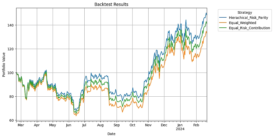

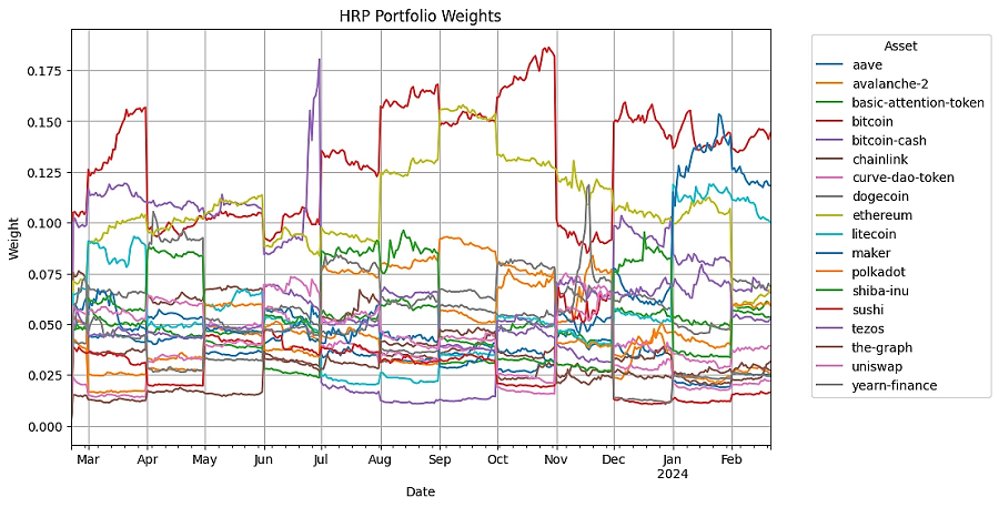
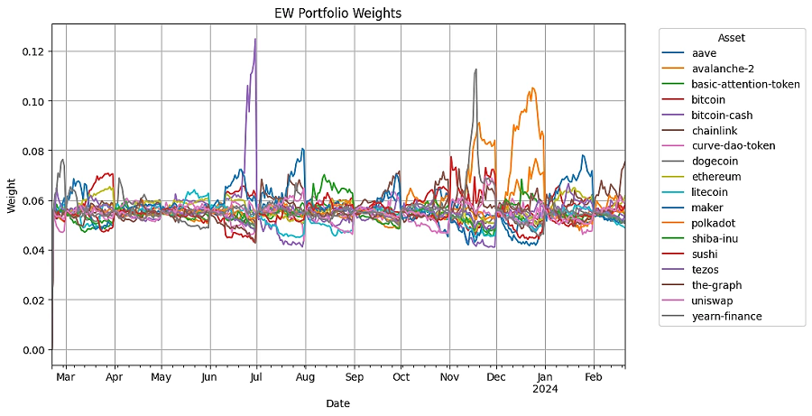
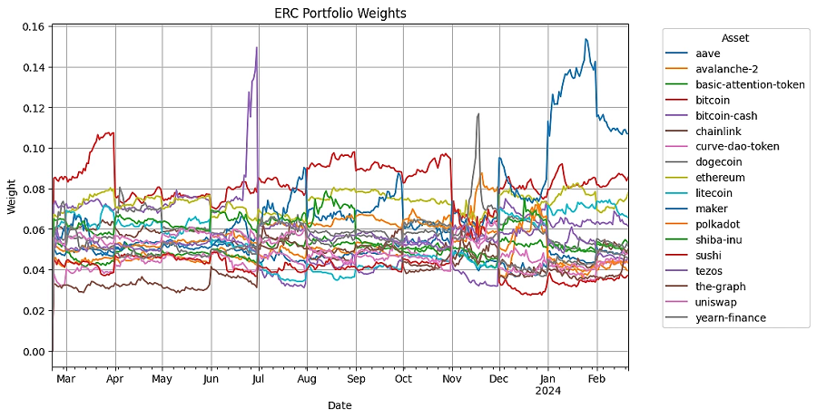
7.4 绘制证券权重

可视化一段时间内的权重分配可以深入了解每种策略如何随市场条件而变化。它有助于理解每种策略的多样化和风险管理方法。

def plot_security_weights(result, name):
    result.get_security_weights().plot(figsize=(10, 6))
    plt.title(f'{name} Portfolio Weights')
    plt.xlabel('Date')
    plt.ylabel('Weight')
    plt.legend(title='Asset', bbox_to_anchor=(1.05, 1), loc='upper left')
    plt.grid()
    plt.show()

输出结果如下：

7.5 回测结果

运行回测后，我们会汇编并显示每个策略的绩效统计数据。这包括总回报、年化回报、最大回撤、夏普比率等指标。比较不同策略的这些指标有助于评估它们的相对绩效和风险特征。

# Compile strategy and benchmark statistics
strategy_performance_stats = pd.concat([
    total_result.stats.iloc[:2],
    total_result.stats.iloc[2:].astype(float)
]).squeeze()

# Compute the Aggregate Random Portfolio statistics
random_performance_stats = pd.concat([
    random_benchmark_results.stats.iloc[:2, 1],
    random_benchmark_results.stats.iloc[2:, 1:].astype(float).mean(axis=1)
])
random_performance_stats.name = 'Aggregate_Random_Portfolio'

# Concatenate the strategy and random portfolio statistics
total_performance_stats = pd.concat([
    strategy_performance_stats,
    random_performance_stats
], axis=1).dropna()

# Function to format as percentage or plain number based on the field type
def format_value(val, as_percentage=False):
    if isinstance(val, pd.Timestamp):
        return val.strftime('%Y-%m-%d')
    try:
        numeric_val = pd.to_numeric(val)
        if pd.isnull(numeric_val):
            return "-"
        return f"{numeric_val * 100:.2f}%" if as_percentage else f"{numeric_val:.2f}"
    except ValueError:
        # Return the value as is if it's not numeric
        return val

# Define the fields that should be formatted as percentages
percentage_fields = [
    'rf', 'total_return', 'cagr', 'max_drawdown', 'mtd', 'three_month',
    'six_month', 'ytd', 'one_year', 'incep', 'daily_mean', 'best_day',
    'worst_day', 'monthly_mean', 'best_month', 'worst_month', 'yearly_mean',
    'best_year', 'worst_year', 'avg_drawdown', 'daily_vol', 'monthly_vol',
    'avg_up_month', 'avg_down_month', 'win_year_perc', 'twelve_month_win_perc'
]

# Copy for formatting
display_performance_stats = total_performance_stats.copy()

# Apply formatting only to numeric fields
for field in display_performance_stats.index:
    if field not in ['Start', 'End']:  # Exclude date fields from numeric formatting
        is_percentage = field in percentage_fields
        display_performance_stats.loc[field] = display_performance_stats.loc[
            field].apply(format_value, as_percentage=is_percentage)

# Rename the indices for display
rename_dict = {
    'start': 'Start',
    'end': 'End',
    'rf': 'Risk-free rate',
    'total_return': 'Total Return',
    'cagr': 'CAGR',
    'max_drawdown': 'Max Drawdown',
    'calmar': 'Calmar Ratio',
    'mtd': 'MTD',
    'three_month': '3m',
    'six_month': '6m',
    'ytd': 'YTD',
    'one_year': '1Y',
    'incep': 'Since Incep. (ann.)',
    'daily_sharpe': 'Daily Sharpe',
    'daily_sortino': 'Daily Sortino',
    'daily_mean': 'Daily Mean (ann.)',
    'daily_vol': 'Daily Vol (ann.)',
    'daily_skew': 'Daily Skew',
    'daily_kurt': 'Daily Kurt',
    'best_day': 'Best Day',
    'worst_day': 'Worst Day',
    'monthly_sharpe': 'Monthly Sharpe',
    'monthly_sortino': 'Monthly Sortino',
    'monthly_mean': 'Monthly Mean (ann.)',
    'monthly_vol': 'Monthly Vol (ann.)',
    'monthly_skew': 'Monthly Skew',
    'monthly_kurt': 'Monthly Kurt',
    'best_month': 'Best Month',
    'worst_month': 'Worst Month',
    'yearly_mean': 'Yearly Mean',
    'best_year': 'Best Year',
    'worst_year': 'Worst Year',
    'avg_drawdown': 'Avg. Drawdown',
    'avg_drawdown_days': 'Avg. Drawdown Days',
    'avg_up_month': 'Avg. Up Month',
    'avg_down_month': 'Avg. Down Month',
    'win_year_perc': 'Win Year %',
    'twelve_month_win_perc': 'Win 12m %'
}

# Apply renaming for readability
display_performance_stats.rename(index=rename_dict, inplace=True)

# Print or return the formatted DataFrame for display
display_performance_stats.loc[[
    'Start', 'End', 'Risk-free rate', 'Total Return', 'CAGR', 'Max Drawdown',
    'Calmar Ratio', 'MTD', '3m', '6m', 'YTD', '1Y', 'Since Incep. (ann.)',
    'Best Day', 'Worst Day', 'Monthly Sharpe', 'Monthly Sortino',
    'Monthly Mean (ann.)', 'Monthly Vol (ann.)', 'Monthly Skew', 'Monthly Kurt',
    'Best Month', 'Worst Month','Avg. Drawdown', 'Avg. Drawdown Days',
    'Avg. Up Month', 'Avg. Down Month'
]]

回测投资组合：

• HRP：分层风险平价
• EW：等权重
• ERC：等风险贡献
• ARP：综合随机投资组合

输出结果如下：

在 2023 年 2 月 20 日至 2024 年 2 月 21 日的一年样本期内，分层风险平价 (HRP) 策略在总回报方面优于等权重 (EW)、等风险贡献 (ERC) 和总随机投资组合 (ARP) 策略，其中 HRP 实现了 48.35% 的回报。它的复合年增长率 (CAGR) 为 48.23%，最大回撤为 -33.78%。虽然 HRP 策略显示出显着的 1.43 的卡尔玛比率和策略中最高的 1.25 的月度夏普比率，表明在样本期内具有良好的风险调整回报，但重要的是要认识到这些结果特定于所分析的时间范围。与其他策略相比，HRP 策略的表现凸显了其在这种特定情况下的有效性，但并不一定意味着在所有市场条件或时间段内都具有整体优势。

7.6 蒙特卡罗假设检验

在假设检验中，我们检查分层风险平价 (HRP) 策略的表现（以月度索提诺比率衡量）是否明显优于从投资组合中选择的随机机会所预期的表现。零假设 (H0) 和备择假设 (Ha) 定义如下：

H0: Strategy's return ≤ 1,000 random portfolios. (μstrategy ≤ μrandom)
Ha: Strategy's return > 1,000 random portfolios. (μstrategy > μrandom)

其中，μstrategy 是投资策略的平均月索提诺比率，μrandom 是随机投资组合的平均月索提诺比率。

# Set the significance level
alpha = 0.05

# Assuming summary_statistics is a DataFrame
summary_statistics = random_benchmark_results.stats

# Extract the monthly_sortino for the investment strategy
investment_strategy_sortino = summary_statistics.loc[
    'monthly_sortino']['Hierachical_Risk_Parity']

# Extract monthly_sortino for all random portfolios for t-test
random_portfolios_sortino = summary_statistics.loc[
    'monthly_sortino'][1:].astype(float).to_numpy()

# Perform a one-sample t-test (one-tailed)
t_statistic, p_value = ttest_1samp(
    random_portfolios_sortino, investment_strategy_sortino)
t_statistic = -t_statistic

# Determine whether the strategy outperformed
outperformed = "outperformed" if p_value < alpha else "did not outperform"

# Output formatted results
print(f"Result: The portfolio {outperformed} the sample of randomly "
      f"generated portfolios based on the monthly_sortino ratio.\n")
print(f"T-statistic: {t_statistic:.4f}")
print(f"P-value (one-tailed): {p_value:.4f}")
print(f"Significance Level: {alpha}\n")

# Plotting histogram and normal distribution
mean = np.mean(random_portfolios_sortino)
std = np.std(random_portfolios_sortino)

# Histogram of Sortino ratios
plt.figure(figsize=(10, 6))
count, bins, ignored = plt.hist(random_portfolios_sortino, 30, density=True,
                                alpha=0.5, edgecolor='black',
                                label='Random Portfolios')

# Normal distribution plot
xmin, xmax = plt.xlim()
x = np.linspace(xmin, xmax, 100)
p = norm.pdf(x, mean, std)
plt.plot(x, p, 'k', linewidth=2)

# Investment strategy's monthly_sortino ratio
plt.axvline(investment_strategy_sortino, color='r', linestyle='dashed',
            linewidth=2, label="Investment Strategy")

# Degrees of freedom
df = len(random_portfolios_sortino) - 1

# Critical t-value for one-tailed test at 95% confidence level
critical_t_value = t.ppf(0.95, df)

# Critical Sortino ratio threshold
critical_ratio_factor = std / np.sqrt(len(random_portfolios_sortino))
critical_sortino = mean + critical_t_value * critical_ratio_factor

plt.axvline(critical_sortino, color='b', linestyle='dashed', linewidth=2,
            label="Critical Sortino Threshold")

plt.title('Distribution of Monthly Sortino Ratios with Critical Threshold')
plt.xlabel('Monthly Sortino Ratio')
plt.ylabel('Density')
plt.legend()

plt.show()

输出结果如下：

Result: The portfolio outperformed the sample of randomly generated portfolios.

T-statistic: 18.0693
P-value (one-tailed): 0.0000
Significance Level: 0.05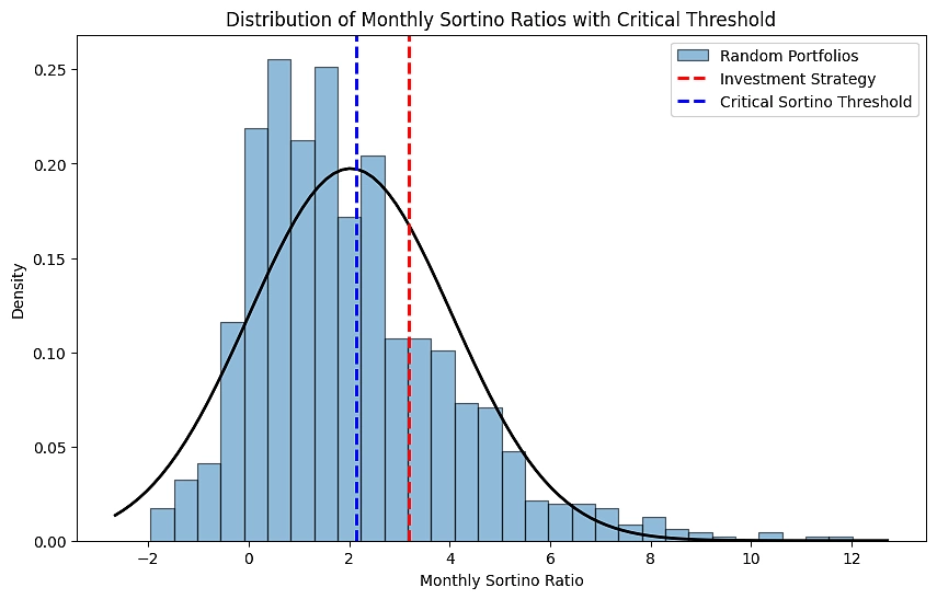

运行测试后，结果显示 p 值为 0.0000，t 统计量为 18.0693。如果我们拒绝原假设，我们断言有足够的证据证明该投资策略的表现优于置信水平为 95% 的随机投资组合。该图进一步证实了这一发现，显示投资策略的索提诺比率明显位于关键索提诺比率阈值和随机投资组合分布的右侧。

# Range of t-values for plotting
t_values = np.linspace(-25, 25, 400)

# PDF of the t-distribution
t_pdf = t.pdf(t_values, df)

# Plotting
plt.figure(figsize=(10, 6))
plt.plot(t_values, t_pdf, label="t-Distribution")

# Fill critical region
plt.fill_between(t_values, 0, t_pdf, where=(t_values > critical_t_value),
                 color='red', alpha=0.5, label="Critical region (alpha=0.05)")

# T-statistic line
plt.axvline(x=t_statistic, color='green', linestyle='--',
            label=f"T-statistic = {t_statistic:.2f}")

# Critical t-value line
plt.axvline(x=critical_t_value, color='black', linestyle='--',
            label=f"Critical t-value = {critical_t_value:.2f}")

plt.legend()
plt.title("Hypothesis Test Visualization")
plt.xlabel("T-value")
plt.ylabel("Probability Density")

plt.show()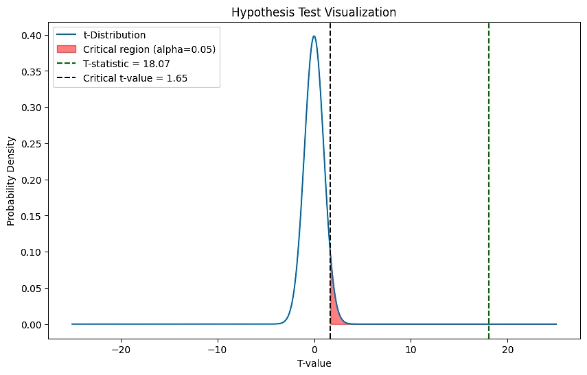

该图直观地显示了分层风险平价 (HRP) 策略表现的假设检验结果。蓝色曲线表示从蒙特卡罗模拟中获得的 t 值的 t 分布。黑色虚线右侧的红色阴影区域表示我们的 alpha 水平 0.05 的临界区域，任何落入该区域的 t 统计量都会导致我们拒绝零假设。我们观察到的 t 统计量（由绿色虚线表示）完全落在临界区域内，证实 HRP 策略的表现在统计上显著高于随机投资组合。临界 t 值为 1.65，高于该值时我们拒绝零假设，而我们的 t 统计量为 18.07，大大超过了这个值，为反对零假设提供了强有力的证据，支持备选假设。

8、自动化策略

本节介绍一个交易机器人，它自动执行分层风险平价策略，将目标分配转换为市场订单，同时管理现有头寸并遵守最低交易门槛。该机器人还具有预览模式，可在执行前验证交易。

8.1 交易机器人

函数 create_positions_dataframe 将账户头寸转换为 Pandas DataFrame。这种标准化格式对于交易机器人根据目标分配评估当前持股至关重要。

def create_positions_dataframe(account_positions):
    temp_df = pd.DataFrame(account_positions)
    columns = [temp_df.iloc[0, i][0] for i in range(len(temp_df.columns))]
    values = [[temp_df.iloc[j, i][1] for i in range(len(temp_df.columns))]
              for j in range(len(temp_df))]
    df_positions = pd.DataFrame(values, columns=columns)
    try:
        df_positions['symbol'] = df_positions['symbol'].apply(
            lambda x: x.split('USD')[0] + '/USD')
        df_positions.set_index('symbol', inplace=True)
        df_positions = df_positions.apply(
            lambda col: pd.to_numeric(col, errors='ignore'))
        return df_positions
    except KeyError:
        return pd.DataFrame(
            columns=['qty', 'side', 'market_value', 'cost_basis']
        )

preview_mode 标志允许用户在不执行真实交易的情况下测试交易机器人，从而提供保障并在实时操作之前验证机器人逻辑的方法。如果 preview_mode 设置为 False，则交易机器人将执行实时订单。请谨慎使用。

preview_mode = True

min_trade_value 设置为 100 美元，表示机器人将忽略低于此金额的任何交易，以确保交易在经济上可行。

min_trade_value = 100  # Minimum dollar value per trade

在这里，我们初始化交易机器人，获取当前账户详细信息和持股情况。它会评估投资组合的价值、现金可用性和购买力。根据我们策略中优化的权重，机器人会准备一份交易清单，考虑最低交易价值阈值，以避免执行经济上不重要的交易。然后，交易机器人会模拟这些交易的执行，提供买入和卖出订单的概览。此模拟允许在实时交易之前进行最终审查，确保与我们的策略和资本配置规则保持一致。

print('Starting Trading Bot...\n')

# Get account details
account = trading_client.get_account()
account = pd.DataFrame(account, columns=['Field', 'Details']).set_index('Field')

# Get portfolio value
portfolio_value = float(account.loc['portfolio_value'].values[0])

# Get current account positions
account_positions = trading_client.get_all_positions()
account_positions = create_positions_dataframe(account_positions)

# Print account details and positions
print(f'Portfolio Value: {f"${portfolio_value:,.2f}"}')
print(f'Cash: ${float(account.loc["cash"].squeeze()):,.2f}')
print(f'Buying Power: ${float(account.loc["buying_power"].squeeze()):,.2f}\n')
if not account_positions.empty:
    print('Account Holdings: \n{}'.format(
        account_positions[['qty', 'side', 'market_value', 'cost_basis']]))
else:
    print('No positions in the portfolio.')

# Define lists to hold sell and buy trade instructions
sell_trades = []
buy_trades = []

# Function to prepare trades based on target and current values
def prepare_trade(symbol, target_value, current_value, current_qty,
                  current_price):
    difference = target_value - current_value
    if difference > 0:
        # Positive difference indicates a buy order
        notional = round(difference, 2)  # Calculate notional value to buy
        if notional >= min_trade_value:  # Skip small value trades
            buy_trades.append((symbol, notional, OrderSide.BUY))
    elif difference < 0:
        # Negative difference indicates a sell order
        notional = round(-difference, 2)  # Calculate notional value to sell
        if notional >= min_trade_value:  # Skip small value trades
            sell_trades.append((symbol, notional, OrderSide.SELL))

# Function to execute or preview trades
def execute_trade(symbol, notional, order_side, preview=True):
    trade_message = (f"{'Preview' if preview else 'Executed'} "
                     f"{order_side.value.lower()} order for "
                     f"{symbol}: Notional ${notional:,.2f}")
    if preview:
        trade_messages.append(trade_message)
    else:
        market_order_data = MarketOrderRequest(
            symbol=symbol,
            notional=notional,
            side=order_side,
            time_in_force=TimeInForce.GTC
        )
        try:
            trading_client.submit_order(order_data=market_order_data)
            trade_messages.append(trade_message)
        except Exception as e:
            trade_messages.append(f"Failed to execute "
                                  f"{order_side.value.lower()} order for "
                                  f"{symbol}: {e}")

print('\nPreparing Trades...\n')

# Collect trades based on current portfolio vs. target weights
for ticker, row in tqdm(weights.iterrows(), total=weights.shape[0]):
    symbol = ticker_mapping.get(ticker)
    if symbol is None:
        print(f"No mapping found for ticker {ticker}")
        continue

    target_weight = row['Optimized Weights']
    target_value = portfolio_value * target_weight

    if symbol in account_positions.index:
        position_row = account_positions.loc[symbol]
        current_value = position_row['market_value']
        current_qty = position_row['qty']
        current_price = current_prices.loc[symbol]
    else:
        current_value = 0
        current_qty = 0
        current_price = 0

    # Prepare trade without executing it immediately
    prepare_trade(symbol, target_value, current_value, current_qty,
                  current_price)

print('\n\nPreviewing Trades...\n' if preview_mode else \
      '\n\nExecuting Trades...\n')

trade_messages = []

for trade in sell_trades + buy_trades:
    execute_trade(*trade, preview=preview_mode)

for message in trade_messages:
    print(message)

print(f'\nTotal Trades: {len(sell_trades) + len(buy_trades)}'
      f'\nSell Trades: {len(sell_trades)}'
      f'\nBuy Trades: {len(buy_trades)}')

print('\nDone!')

输出结果如下：

Starting Trading Bot...

Portfolio Value: $102,198.99
Cash: $14,678.53
Buying Power: $29,357.06

Account Holdings: 
                    qty               side  market_value    cost_basis
symbol                                                                
AAVE/USD      53.031986  PositionSide.LONG   5449.036580   4873.639530
AVAX/USD      56.150439  PositionSide.LONG   2166.845424   2175.267990
BAT/USD    13704.653261  PositionSide.LONG   3705.436739   3453.435575
BCH/USD       20.679385  PositionSide.LONG   5605.560950   5374.841049
BTC/USD        0.304311  PositionSide.LONG  16271.957289  15619.655041
CRV/USD    10941.174129  PositionSide.LONG   6583.960944      0.000000
DOGE/USD   34293.311273  PositionSide.LONG   2987.156601   2956.426365
DOT/USD      463.152266  PositionSide.LONG   3719.112695      0.000000
ETH/USD        2.761884  PositionSide.LONG   8713.744512   8071.661684
GRT/USD     7204.676907  PositionSide.LONG   2120.480507   1720.671372
LINK/USD     277.058115  PositionSide.LONG   5253.215799   5090.194804
LTC/USD      101.623754  PositionSide.LONG   7216.099548   7009.420266
SUSHI/USD   2899.258768  PositionSide.LONG   4541.109008   3664.692075
UNI/USD      682.816928  PositionSide.LONG   7777.284814   5011.261719
XTZ/USD     4775.295230  PositionSide.LONG   5409.454436      0.000000

Preparing Trades...

100%|██████████| 18/18 [00:00<00:00, 4038.16it/s]

Previewing Trades...

Preview sell order for BTC/USD: Notional $7,400.06
Preview sell order for ETH/USD: Notional $1,535.29
Preview sell order for UNI/USD: Notional $1,379.63
Preview sell order for CRV/USD: Notional $2,612.51
Preview sell order for BCH/USD: Notional $1,760.83
Preview sell order for SUSHI/USD: Notional $1,314.69
Preview buy order for DOT/USD: Notional $3,700.53
Preview buy order for DOGE/USD: Notional $4,011.43
Preview buy order for XTZ/USD: Notional $1,474.67
Preview buy order for SHIB/USD: Notional $6,725.72
Preview buy order for BAT/USD: Notional $2,669.74
Preview buy order for AAVE/USD: Notional $231.18
Preview buy order for YFI/USD: Notional $4,696.04
Preview buy order for MKR/USD: Notional $4,313.82
Preview buy order for AVAX/USD: Notional $2,091.79
Preview buy order for GRT/USD: Notional $711.45

Total Trades: 16
Sell Trades: 6
Buy Trades: 10

Done!

交易机器人启动时显示投资组合价值 102,198.99 美元，其中现金 14,678.53 美元，可用购买力 29,357.06 美元。当前账户持有量分散在各种加密货币中，比特币在投资组合中市值最高。该机器人将预览 16 笔交易，包括 6 笔卖出和 10 笔买入，交易决策基于优化投资组合权重。值得注意的是，最大的预期交易是比特币的卖单，名义价值为 7,400.06 美元，这表明该机器人能够处理大量交易。交易预览成功结束会话，表明已准备好实际执行，等待确认。

9、风险、注意事项和结论

算法交易虽然提供了许多好处，例如速度、效率和消除情绪化决策，但也存在一系列风险和注意事项。一个关键风险涉及过度拟合的可能性，即策略可能在历史数据上表现异常出色，但无法准确预测未来走势。这尤其适用于基于机器学习的策略，例如分层风险平价 (HRP)，如果未经适当验证，它可能会将噪音捕获为信号。

机器学习在金融领域的吸引力有时会掩盖这些算法的固有局限性。对任何交易策略保持科学的怀疑态度至关重要，无论其复杂性或所涉及算法的复杂程度如何。机器学习模型（包括 HRP）的成功在很大程度上取决于它们所训练数据的质量和相关性，并且它们的性能可能会受到市场条件、经济结构变化或监管环境的显著影响。

交易机器人虽然功能强大，但在其编程的约束下运行。它们缺乏人类的判断能力和基于情境的决策能力，有时会导致意外交易或无法适应新的市场条件。此外，连接问题、系统崩溃或软件错误等技术问题可能会导致交易错过或订单重复。此外，金融市场受到无数难以量化的因素的影响，例如政治事件、消费者行为的变化或新技术的出现。这些因素可能会导致机器学习模型或交易机器人从未遇到过的情况，从而可能导致次优决策。

总之，虽然机器学习和算法交易策略（如 HRP）对投资者来说是有价值的工具，但它们不应被视为万无一失的解决方案。交易者必须尽职尽责、持续监控和对样本外数据进行严格的回测，以确保这些策略在各种市场条件下保持稳健。制定风险管理协议也很重要，以便在策略表现不如预期时减轻潜在损失。

原文链接：Crypto Machine Learning: Develop a Crypto Algorithmic Trading Strategy with Python

DefiPlot翻译整理，转载请标明出处